The Implied Volatility Surface: What Skew and Term Structure Actually Tell You

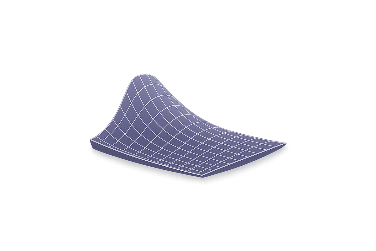
Implied volatility is not observed directly anywhere. It is backed out of an option's market price by solving the Black-Scholes-Merton formula in reverse. The model normally runs forward: feed in spot, strike, time to expiration, the risk-free rate, and volatility, and it outputs a theoretical option price. To get implied volatility, you invert that process — you take the option's actual traded price (typically the bid/ask midpoint) as a given, hold every other input fixed at its known market value, and solve for the one input you don't otherwise have: volatility.

Because the BSM formula has no closed-form algebraic inverse for volatility, this solve is done numerically, almost universally with Newton-Raphson iteration: start with a volatility guess, compute the model price and its sensitivity to volatility (vega), use that to refine the guess, and repeat until the model price converges to the observed market price within a small tolerance. Every options data provider and broker platform runs this same basic solve independently on every strike and expiration it quotes, which is exactly how a full chain's worth of implied volatilities gets produced from a chain's worth of raw quotes.

This is a fundamentally different computation from realized (historical) volatility. Realized volatility is computed directly from a time series of the underlying's past returns — typically the annualized standard deviation of log returns over some lookback window. It requires no option prices and no model inversion at all; it is a statistical property of price history. Implied volatility, by contrast, requires no return history whatsoever — it requires an option price and a pricing model, and what it measures is not what already happened to the underlying but what the market is currently paying for, expressed in volatility terms. The two will frequently diverge, and the gap between them (the volatility risk premium) is itself a tradeable signal, but they are not two ways of measuring the same underlying quantity.

This distinction matters here because of what comes next: each point on an option chain gets its own independent IV solve, anchored to that specific contract's own market price. A $50 call expiring in two weeks and a $55 call expiring in two months are two separate solves against two separate prices. There is no mechanical reason for these independent solves to return the same number — and the patterns in where they systematically differ are exactly what skew and term structure describe.

A single Black-Scholes implied volatility number describes one option, at one strike, at one expiration. The moment you look across strikes or across expirations simultaneously, that number stops behaving like a constant. It varies systematically — and that variation is not noise. It is priced information about how the market expects the underlying's return distribution to behave, and it is the single richest dataset available to a retail options trader who knows how to read it.

This article builds the implied volatility surface dimension by dimension: first across strikes (skew), then across expirations (term structure), then as a joint object, and finally covers what changes in surface shape mean for a position you are already holding.

Why one IV number isn't enough

The Black-Scholes-Merton model assumes the underlying follows geometric Brownian motion with constant volatility. Under that assumption, every option on the same underlying, regardless of strike or expiration, should produce the same implied volatility once solved. In practice, this almost never holds. The BSM formula remains popular with practitioners largely as a convenient mapping device from option prices to a single real number called implied volatility, which allows easier comparison across strikes, expiries, and underlying assets — not because the model's constant-volatility assumption is realistic.

Once you compute IV for every traded strike and expiration on an underlying, you get a two-dimensional object: IV as a function of strike (K) and time to expiration (T). The general pattern is that implied volatility decreases as moneyness approaches one and increases as it moves further away — commonly called the volatility smile or volatility skew. Adding time to expiration as a second dimension turns that smile into a full surface.

Two cross-sections of this surface matter most for a trader:

• Fix T, vary K → the skew (or smile) for one expiration.
• Fix K (or fixed moneyness), vary T → the term structure.

Skew: the strike dimension

For equity index options, the skew is consistently downward-sloping rather than symmetric: out-of-the-money puts carry higher implied volatility than out-of-the-money calls at the same distance from spot. This pattern has been shown to be directly related to the conditional non-normality of the underlying's risk-neutral return distribution — a smile reflects fat tails in the distribution, while a skew reflects asymmetry in it.

Two complementary explanations are standard in the literature:

1. Leverage effect. As an equity price falls, the firm's leverage ratio rises mechanically (same debt, less equity value), which increases the equity's volatility. This creates a structural reason for downside volatility to run higher than upside volatility, independent of any crash expectation.
2. Crash risk premium. Demand for downside protection (institutional hedging, portfolio insurance) bids up OTM put prices beyond what the leverage effect alone would justify, since investors are willing to pay a premium for a payoff that performs precisely when everything else underperforms.

Single-name skew is typically flatter than index skew, since idiosyncratic crash risk is harder to hedge collectively and earnings-related uncertainty can cut in either direction.

Reading skew steepness. A standard normalization is the 25-delta risk reversal: the IV of a 25-delta put minus the IV of a 25-delta call, for the same expiration. A more negative number (relatively) means richer puts and a steeper skew — consistent with either a higher embedded crash premium or compressed realized volatility in spot, making downside convexity comparatively cheap to own as you approach the event. Skew steepening into a known catalyst (an index rebalance, a macro print, an election) is a frequently cited pattern; skew flattening after the event resolves is the corresponding mean-reversion.

Term structure: the maturity dimension

Term structure describes how at-the-money (or fixed-delta) implied volatility varies across expirations, holding strike-relative-to-spot constant. If skew describes the surface zoomed into a single expiration, term structure describes the same surface viewed across all expirations at once.

Two regimes recur:

• Contango: longer-dated IV trades above near-dated IV. This is the typical resting state, reflecting greater cumulative uncertainty over a longer horizon and a baseline term premium.
• Backwardation: near-dated IV trades above longer-dated IV. This shows up around concentrated event risk — earnings, FOMC, a binary catalyst — where the market prices a near-term volatility spike that is expected to fade once the event passes.

The clearest public example is the VIX term structure itself, which sits in contango most of the time and flips to backwardation during acute stress, when near-term realized and implied volatility spike faster than the market's longer-run volatility expectation.

For single-name options, the same mechanic plays out around earnings: the front expiration that straddles the earnings date trades at an elevated IV relative to the back-month expiration that doesn't, because almost all of the uncertainty resolves on one specific date rather than smoothly over the option's life. ORATS' own surface construction explicitly separates this earnings effect from the smooth 30-day-to-2-year term structure baseline, treating the event-driven component as a distinct input rather than folding it into a single decay curve.

The joint surface: why this matters for your existing position

Skew and term structure aren't independent facts you memorize once and forget — the surface moves as spot moves, and how it moves changes your actual P&L. This is where two competing models of IV dynamics become directly relevant to a position you're holding.

Under the "sticky strike" rule, the implied volatility for an option at a given strike and maturity is treated as independent of the underlying's price — it stays pinned to that strike. Under the competing "sticky delta" (or sticky moneyness) rule, implied volatility is instead treated as a function of moneyness, so the IV attached to, say, the 25-delta option stays roughly constant even as spot moves and a different strike becomes the 25-delta option.

The distinction is not academic. Under sticky strike, an option's delta matches the standard Black-Scholes delta computed at the prevailing volatility. Under sticky delta, the effective delta of a position is higher than the Black-Scholes delta for any option with positive vega — because as spot moves toward a strike, that strike's "skew-implied" IV moves with it, adding an extra component to the option's price sensitivity that pure BSM delta doesn't capture.

Practically: if you're short a downside put and spot drops toward your strike, sticky-delta dynamics mean the IV at that strike rises as it becomes more at-the-money — compounding your delta losses with a vega loss at the same time. A sticky-strike assumption would have left that specific strike's IV unchanged. Which regime dominates is empirically a mixed picture and varies by underlying and regime — one study using IBEX 35 monthly surfaces found the sticky strike rule fit better when the underlying displayed no clear trend, with both rules describing the surface's evolution reasonably well overall. The practical takeaway isn't to pick one model as universally correct — it's to recognize that your realized Greeks during a fast move will diverge from your static, single-snapshot Greeks, and the direction of that divergence depends on which regime the surface is currently behaving like.

A related, more mechanical phenomenon sits underneath both: large concentrations of open interest at specific strikes create gamma hedging flows that can anchor spot near those strikes as expiration approaches — what's often called "pinning." When gamma is high at a heavily traded strike, market-maker hedging flows can become self-reinforcing, pulling or holding the underlying price near that level as positions are continuously rehedged. This is a separate effect from sticky-strike/sticky-delta dynamics but tends to show up in the same conversations, since both relate strike-level positioning to how price and volatility co-move.

Practical reads, without full surface calibration

You don't need to fit a parametric surface model to extract signal from its shape. A few checks are accessible with nothing more than a chain snapshot:

• Skew level vs. its own history. Compare today's 25-delta risk reversal to its trailing distribution for the same underlying. Skew sitting in the top decile of its own range is a different signal than an absolute skew number compared across unrelated names.
• Term structure shape around known events. Backwardation into an earnings date is expected; backwardation with no scheduled catalyst is informative on its own, since it implies the market is pricing near-term risk it hasn't told you the source of.
• Skew and term structure moving together vs. independently. Skew steepening alongside front-month IV spiking (backwardation) is a classic pre-event signature. Skew steepening with flat term structure is a different, more structural statement about the distribution of outcomes rather than a single-date catalyst.

None of this requires fitting a stochastic volatility model. It requires comparing today's surface cross-sections to their own recent history — which is itself a backtesting question, not a calibration question.

A note on calibrated surface models

Production systems that need a full, arbitrage-free surface — rather than a handful of cross-sections — typically fit a parametric or semi-parametric model to the observed quotes. The SVI (Stochastic Volatility Inspired) parameterization is the most widely used in practice for fitting a single expiration's smile, with separate term-structure interpolation layered on top to connect expirations into a complete surface. Covering SVI's parameter fitting in depth is outside the scope of this piece; it's referenced here only as the natural next step if you want to move from reading surface shape to reconstructing the full surface programmatically.

Reading skew and term structure shape by hand is a reasonable starting point. Testing whether a given surface signal actually has predictive value for a strategy requires backtesting it against historical data — which is what Quantropy AI is built for. → Join the waitlist at quantropy.ai

Sources

1. Vanderhoek, R. et al. "A new encoding of implied volatility surfaces for their synthetic generation." arXiv:2211.12892. https://arxiv.org/pdf/2211.12892
2. Various authors. "Implied Volatility Surface: Construction Methodologies and Characteristics." arXiv:1107.1834. https://arxiv.org/pdf/1107.1834
3. Daglish, T., Hull, J., Suo, W. "Volatility Surfaces: Theory, Rules of Thumb, and Empirical Evidence." University of Toronto. https://www-2.rotman.utoronto.ca/~hull/downloadablepublications/DaglishHullSuoRevised.pdf
4. Alonso, F. et al. "Dynamics of the Implied Volatility Surface: Theory and Empirical Evidence." https://archivo.alde.es/encuentros.alde.es/anteriores/xiiieea/trabajos/pdf/079.pdf
5. MenthorQ. "Sticky Strikes and the Skew in Options Trading Guide." https://menthorq.com/guide/sticky-strikes-and-the-skew-in-options-trading/